How To Use FB Prophet for Time-series Forecasting: Vehicle Traffic Volume
Recently, I came across a few articles mentioning Facebook’s Prophet library that looked interesting (although the initial release was almost 3 years ago!), so I decided to dig more into it.
Prophet is an open-source library developed by Facebook which aims to make time-series forecasting easier and more scalable. It is a type of generalized additive model (GAM), which uses a regression model with potentially non-linear smoothers. It is called additive because it adds multiple decomposed parts to explain some trends. For example, Prophet uses the following components:
\[y(t) = g(t) + s(t) + h(t) + e(t)\]where,
$g(t)$: Growth. Big trend. Non-periodic changes.
$s(t)$: Seasonality. Periodic changes (e.g. weekly, yearly, etc.) represented by Fourier Series.
$h(t)$: Holiday effect that represents irregular schedules.
$e(t)$: Error. Any idiosyncratic changes not explained by the model.
In this post, I will explore main concepts and API endpoints of the Prophet library.
Table of Contents
- Prepare Data
- Train And Predict
- Check Components
- Evaluate
- Trend Change Points
- Seasonality Mode
- Saving Model
- References
1. Prepare Data
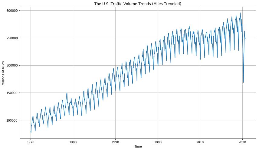
In this post. We will use the U.S. traffic volume data available here, which is a monthly traffic volume (miles traveled) on public roadways from January 1970 until September 2020. The unit is a million miles.
import pandas as pd
import matplotlib.pyplot as plt

# to mute Pandas warnings Prophet needs to fix
import warnings
warnings.simplefilter(action='ignore', category=FutureWarning)
df.head()
| DATE | TRFVOLUSM227NFWA | |
|---|---|---|
| 0 | 1970-01-01 | 80173.0 |
| 1 | 1970-02-01 | 77442.0 |
| 2 | 1970-03-01 | 90223.0 |
| 3 | 1970-04-01 | 89956.0 |
| 4 | 1970-05-01 | 97972.0 |
Prophet is hard-coded to use specific column names; ds for dates and y for the target variable we want to predict.
# Prophet requires column names to be 'ds' and 'y'
df.columns = ['ds', 'y']
# 'ds' needs to be datetime object
df['ds'] = pd.to_datetime(df['ds'])
When plotting the original data, we can see there is a big, growing trend in the traffic volume, although there seems to be some stagnant or even decreasing trends (change of rate) around 1980, 2008, and most strikingly, 2020 . Checking how Prophet can handle these changes would be interesting. There is also a seasonal, periodic trend that seems to repeat each year. It goes up until the middle of the year and goes down again. Will Prophet capture this as well?
For train test split, do not forget that we cannot do a random split for time-series data. We use ONLY the earlier part of data for training and the later part of data for testing given a cut-off point. Here, we use 2019/1/1 as our cut-off point.
# split data
train = df[df['ds'] < pd.Timestamp('2019-01-01')]
test = df[df['ds'] >= pd.Timestamp('2019-01-01')]
print(f"Number of months in train data: {len(train)}")
print(f"Number of months in test data: {len(test)}")
    Number of months in train data: 588
    Number of months in test data: 21
2. Train And Predict
Let’s train a Prophet model. You just initialize an object and fit! That’s all.
Prophet warns that it disabled weekly and daily seasonality. That’s fine because our data set is monthly so there is no weekly or daily seasonality.
from fbprophet import Prophet

# fit model - ignore train/test split for now
m = Prophet()
m.fit(train)
    INFO:fbprophet:Disabling weekly seasonality. Run prophet with weekly_seasonality=True to override this.
    INFO:fbprophet:Disabling daily seasonality. Run prophet with daily_seasonality=True to override this.

    <fbprophet.forecaster.Prophet at 0x121b8dc88>
When making predictions with Prophet, we need to prepare a special object called future dataframe. It is a Pandas DataFrame with a single column ds that includes all datetime within the training data plus additional periods given by user.
The parameter periods is basically the number of points (rows) to predict after the end of the training data. The
interval (parameter freq) is set to ‘D’ (day) by default, so we need to adjust it to ‘MS’ (month start) as our data
is monthly. I set periods=21 as it is the number of points in the test data.
# future dataframe - placeholder object
future = m.make_future_dataframe(periods=21, freq='MS')
# start of the future df is same as the original data
future.head()
| ds | |
|---|---|
| 0 | 1970-01-01 |
| 1 | 1970-02-01 |
| 2 | 1970-03-01 |
| 3 | 1970-04-01 |
| 4 | 1970-05-01 |
# end of the future df is original + 21 periods (21 months)
future.tail()
| ds | |
|---|---|
| 604 | 2020-05-01 |
| 605 | 2020-06-01 |
| 606 | 2020-07-01 |
| 607 | 2020-08-01 |
| 608 | 2020-09-01 |
It’s time to make actual predictions. It’s simple - just predict with the placeholder DataFrame future.
# predict the future
forecast = m.predict(future)
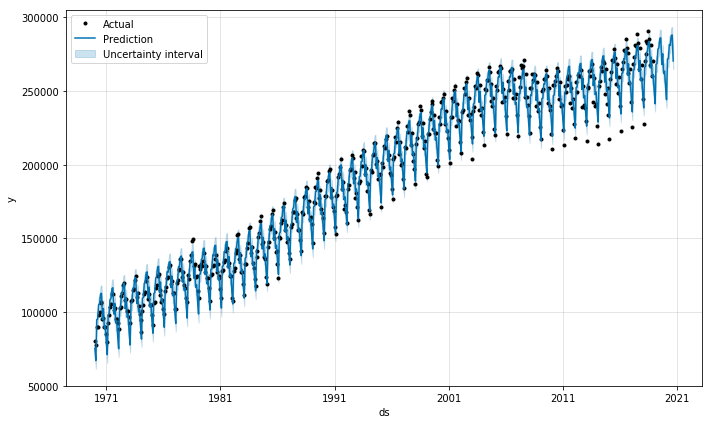
Prophet has a nice built-in plotting function to visualize forecast data. Black dots are for actual data and the blue line is prediction. You can also use matplotlib functions to adjust the figure, such as adding legend or adding xlim or ylim.
# Prophet's own plotting tool to see
fig = m.plot(forecast)
plt.legend(['Actual', 'Prediction', 'Uncertainty interval'])
plt.show()
3. Check Components
So, what is in the forecast DataFrame? Let’s take a look.
forecast.head()
| ds | trend | yhat_lower | yhat_upper | trend_lower | trend_upper | additive_terms | additive_terms_lower | additive_terms_upper | yearly | yearly_lower | yearly_upper | multiplicative_terms | multiplicative_terms_lower | multiplicative_terms_upper | yhat | |
|---|---|---|---|---|---|---|---|---|---|---|---|---|---|---|---|---|
| 0 | 1970-01-01 | 94281.848744 | 69838.269924 | 81366.107613 | 94281.848744 | 94281.848744 | -18700.514310 | -18700.514310 | -18700.514310 | -18700.514310 | -18700.514310 | -18700.514310 | 0.0 | 0.0 | 0.0 | 75581.334434 |
| 1 | 1970-02-01 | 94590.609819 | 61661.016554 | 73066.758942 | 94590.609819 | 94590.609819 | -27382.307301 | -27382.307301 | -27382.307301 | -27382.307301 | -27382.307301 | -27382.307301 | 0.0 | 0.0 | 0.0 | 67208.302517 |
| 2 | 1970-03-01 | 94869.490789 | 89121.298723 | 99797.427717 | 94869.490789 | 94869.490789 | 37.306077 | 37.306077 | 37.306077 | 37.306077 | 37.306077 | 37.306077 | 0.0 | 0.0 | 0.0 | 94906.796867 |
| 3 | 1970-04-01 | 95178.251864 | 89987.904019 | 101154.016322 | 95178.251864 | 95178.251864 | 166.278079 | 166.278079 | 166.278079 | 166.278079 | 166.278079 | 166.278079 | 0.0 | 0.0 | 0.0 | 95344.529943 |
| 4 | 1970-05-01 | 95477.052904 | 99601.487207 | 110506.849617 | 95477.052904 | 95477.052904 | 9672.619044 | 9672.619044 | 9672.619044 | 9672.619044 | 9672.619044 | 9672.619044 | 0.0 | 0.0 | 0.0 | 105149.671948 |
There are many components in it but the main thing that you would care about is yhat which has the final predictions. _lower and _upper flags are for uncertainty intervals.
- Final predictions:
yhat,yhat_lower, andyhat_upper
Other columns are components that comprise the final prediction as we discussed in the introduction. Let’s compare Prophet’s components and what we see in our forecast DataFrame.
\[y(t) = g(t) + s(t) + h(t) + e(t)\]- Growth ($g(t)$):
trend,trend_lower, andtrend_upper - Seasonality ($s(t)$):
additive_terms,additive_terms_lower, andadditive_terms_upper- Yearly seasonality:
yearly,yearly_lower, andyearly_upper
- Yearly seasonality:
The additive_terms represent the total seasonality effect, which is the same as yearly seasonality as we disabled weekly and daily seasonalities. All multiplicative_terms are zero because we used additive seasonality mode by default instead of multiplicative seasonality mode, which I will explain later.
Holiday effect ($h(t)$) is not present here as it’s yearly data.
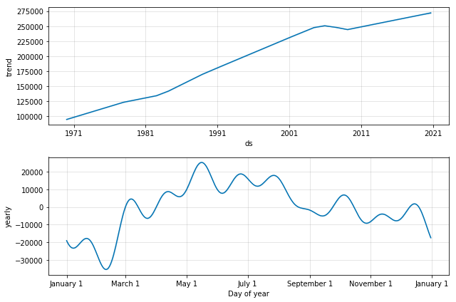
Prophet also has a nice built-in function for plotting each component. When we plot our forecast data, we see two components; general growth trend and yearly seasonality that appears throughout the years. If we had more components such as weekly or daily seasonality, they would have been presented here as well.
# plot components
fig = m.plot_components(forecast)
4. Evaluate
4.1. Evaluate the model on one test set
How good is our model? One way we can understand the model performance, in this case, is to simply calculate the root mean squared error (RMSE) between the actual and predicted values of the above test period.
from statsmodels.tools.eval_measures import rmse

predictions = forecast.iloc[-len(test):]['yhat']
actuals = test['y']

print(f"RMSE: {round(rmse(predictions, actuals))}")
RMSE: 32969.0
However, this probably under-represents the general model performance because our data has a drastic change in the middle of the test period which is a pattern that has never been seen before. If our data was until 2019, the model performance score would have been much higher.
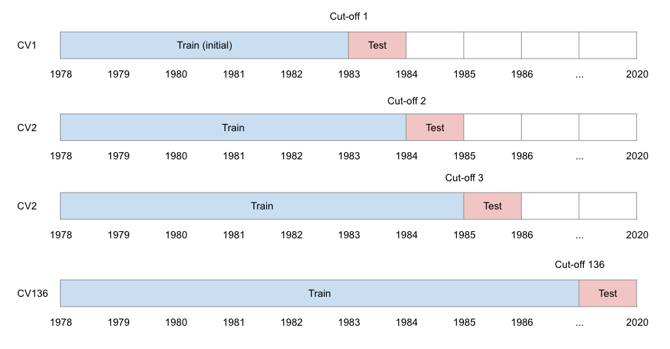
4.2. Cross validation
Alternatively, we can perform cross-validation. As previously discussed, time-series analysis strictly uses train data whose time range is earlier than that of test data. Below is an example where we use 5 years of train data to predict 1-year of test data. Each cut-off point is equally spaced with 1 year gap.
Prophet also provides built-in model diagnostics tools to make it easy to perform this cross-validation. You just need to define three parameters: horizon, initial, and period. The latter two are optional.
- horizon: test period of each fold
- initial: minimum training period to start with
- period: time gap between cut-off dates
Make sure to define these parameters in string and in this format: ‘X unit’. X is the number and unit is ‘days’ or
‘secs’, etc. that is compatible with pd.Timedelta. For example, 10 days.
You can also define parallel to make the cross validation faster.
from fbprophet.diagnostics import cross_validation

# test period
horizon = '365 days'

# itraining period (optional. default is 3x of horizon)
initial = str(365 * 5) + ' days'

# spacing between cutoff dates (optional. default is 0.5x of horizon)
period = '365 days'

df_cv = cross_validation(m, initial=initial, period=period, horizon=horizon, parallel='processes')
    INFO:fbprophet:Making 43 forecasts with cutoffs between 1975-12-12 00:00:00 and 2017-12-01 00:00:00
    INFO:fbprophet:Applying in parallel with <concurrent.futures.process.ProcessPoolExecutor object at 0x12fb4d3c8>
This is the predicted output using cross-validation. There can be many predictions for the same timestamp if period
is smaller than horizon.
# predicted output using cross validation
df_cv
| ds | yhat | yhat_lower | yhat_upper | y | cutoff | |
|---|---|---|---|---|---|---|
| 0 | 1976-01-01 | 102282.737592 | 100862.769604 | 103589.684840 | 102460.0 | 1975-12-12 |
| 1 | 1976-02-01 | 96811.141761 | 95360.095284 | 98247.364027 | 98528.0 | 1975-12-12 |
| 2 | 1976-03-01 | 112360.483572 | 110908.136982 | 113775.264669 | 114284.0 | 1975-12-12 |
| 3 | 1976-04-01 | 112029.016859 | 110622.916037 | 113458.999123 | 117014.0 | 1975-12-12 |
| 4 | 1976-05-01 | 119161.998160 | 117645.653475 | 120579.267732 | 123278.0 | 1975-12-12 |
| ... | ... | ... | ... | ... | ... | ... |
| 511 | 2018-08-01 | 279835.003826 | 274439.830747 | 285259.974314 | 284989.0 | 2017-12-01 |
| 512 | 2018-09-01 | 261911.246557 | 256328.677902 | 267687.122886 | 267434.0 | 2017-12-01 |
| 513 | 2018-10-01 | 268979.448383 | 263001.411543 | 274742.978202 | 281382.0 | 2017-12-01 |
| 514 | 2018-11-01 | 255612.520483 | 249813.339845 | 261179.979649 | 260473.0 | 2017-12-01 |
| 515 | 2018-12-01 | 257049.510224 | 251164.508448 | 263062.671327 | 270370.0 | 2017-12-01 |
516 rows × 6 columns
Below are different performance metrics for different rolling windows. As we did not define any rolling window, Prophet went ahead and calculated many different combinations and stacked them up in rows (e.g. 53 days, …, 365 days). Each metric is first calculated within each rolling window and then averaged across many available windows.
from fbprophet.diagnostics import cross_validation, performance_metrics

# performance metrics
df_metrics = performance_metrics(df_cv)  # can define window size, e.g. rolling_window=365
df_metrics
| horizon | mse | rmse | mae | mape | mdape | coverage | |
|---|---|---|---|---|---|---|---|
| 0 | 53 days | 3.886562e+07 | 6234.229883 | 5143.348348 | 0.030813 | 0.027799 | 0.352941 |
| 1 | 54 days | 3.983610e+07 | 6311.584390 | 5172.484468 | 0.030702 | 0.027799 | 0.372549 |
| 2 | 55 days | 4.272605e+07 | 6536.516453 | 5413.997433 | 0.031607 | 0.030305 | 0.352941 |
| 3 | 56 days | 4.459609e+07 | 6678.030078 | 5662.344846 | 0.032630 | 0.031911 | 0.313725 |
| 4 | 57 days | 4.341828e+07 | 6589.254589 | 5650.202377 | 0.032133 | 0.031481 | 0.313725 |
| ... | ... | ... | ... | ... | ... | ... | ... |
| 115 | 361 days | 2.880647e+07 | 5367.165528 | 3960.025025 | 0.020118 | 0.015177 | 0.607843 |
| 116 | 362 days | 3.158472e+07 | 5620.028791 | 4158.035261 | 0.020836 | 0.015177 | 0.588235 |
| 117 | 363 days | 3.798731e+07 | 6163.384773 | 4603.360382 | 0.022653 | 0.017921 | 0.549020 |
| 118 | 364 days | 4.615621e+07 | 6793.836092 | 4952.443173 | 0.023973 | 0.018660 | 0.529412 |
| 119 | 365 days | 5.428934e+07 | 7368.129817 | 5262.131511 | 0.024816 | 0.018660 | 0.529412 |
120 rows × 7 columns
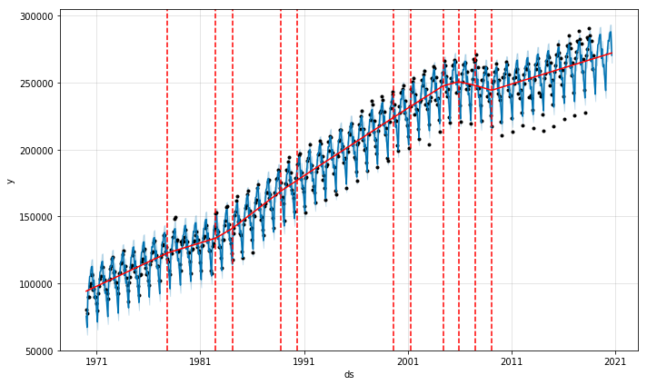
5. Trend Change Points
Another interesting functionality of Prophet is add_changepoints_to_plot. As we discussed in the earlier sections, there are a couple of points where the growth rate changes. Prophet can find those points automatically and plot them!
from fbprophet.plot import add_changepoints_to_plot

# plot change points
fig = m.plot(forecast)
a = add_changepoints_to_plot(fig.gca(), m, forecast)
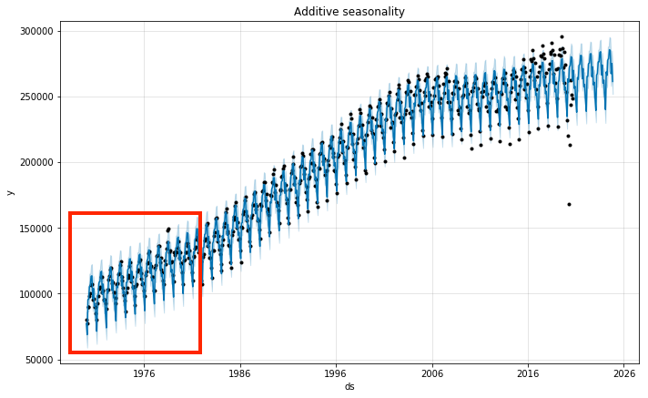
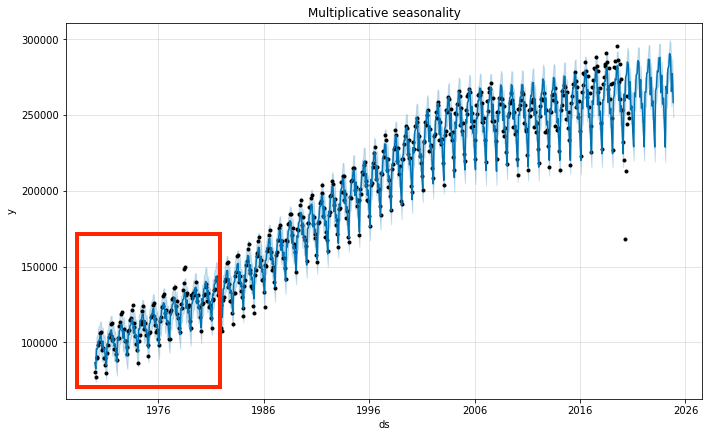
6. Seasonality Mode
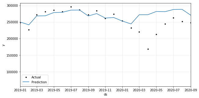
The growth in trend can be additive (rate of change is linear) or multiplicative (rate changes over time). When you
see the original data, the amplitude of seasonality changes - smaller in the early years and
bigger in the later years. So, this would be a multiplicative growth case rather than an additive growth case. We
can adjust the seasonality parameter so we can take into account this effect.
# additive mode
m = Prophet(seasonality_mode='additive')
# multiplicative mode
m = Prophet(seasonality_mode='multiplicative')
You can see that the blue lines (predictions) are more in line with the black dots (actuals) when in multiplicative seasonality mode.
7. Saving Model
We can also easily export and load the trained model as json.
import json
from fbprophet.serialize import model_to_json, model_from_json

# Save model
with open('serialized_model.json', 'w') as fout:
    json.dump(model_to_json(m), fout)

# Load model
with open('serialized_model.json', 'r') as fin:
    m = model_from_json(json.load(fin))